 Products Home / Technical Resources / Beam Characterization Tutorials / Optical Spectrum Analyzer Tutorials
Optical Spectrum Analyzer Tutorials

Please Wait

Design
This tab describes the key concepts and implementation of the design used in Thorlabs' Fourier Transform Optical Spectrum Analyzers.
Contents- Interferometer Design
- Resolution and Sensitivity
- Absolute Power and Power Density
- Interferogram Data Acquisition
- Interferogram Data Processing
- Wavelength Meter Mode
- Wavelength Calibration and Accuracy
- Optical Rejection Ratio
Click to Enlarge
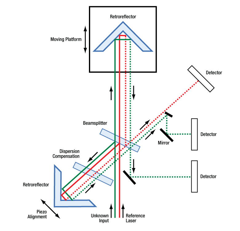
Figure 1.2 Schematic of the optical path in Thorlabs' Redstone OSA. Note that the OSA302 does not include the dispersion compensation plate in the interferometer.
Click to Enlarge
Figure 1.1 Schematic of the optical path in Thorlabs' OSA20xC OSAs, detailing the dual retroreflector design.
Interferometer Design
Thorlabs' OSA20xC Fourier Transform Optical Spectrum Analyzers (FT-OSA) utilize two retroreflectors, as shown in Figure 1.1. These retroreflectors are mounted on a voice-coil-driven platform, which dynamically changes the optical path length of the two arms of the interferometer simultaneously and in opposite directions. The advantage of this layout is that it changes the optical path difference (OPD) of the interferometer by four times the mechanical movement of the platform. The longer the change in OPD, the finer the spectral detail the FT-OSA can resolve.
The Redstone® OSA30x FT-OSA uses a standard arrangement of one fixed and one movable retroreflector as shown in Figure 1.2. The mobile retroreflector is mounted on Thorlabs' patented voice-coil-driven platform*, which changes the optical path length of the branch. The fixed retroreflector is mounted on a piezo actuator that translates the retroreflector in the two dimensions orthogonal to the beam path in a self-alignment algorithm. This configuration changes the OPD between the two branches by twice the mechanical movement of the platform.
*The Redstone OSA30x is constructed using Thorlabs' patented voice-coil-driven platform design.
After collimating the unknown input, a beamsplitter divides the optical signal into two separate paths. The path length difference between the two paths is varied up to 40 mm for the OSA20xC and 160 mm for the Redstone. The collimated light fields then optically interfere as they recombine at the beamsplitter.
The detector assemblies shown in Figures 1.1 and 1.2 record the interference pattern, commonly referred to as an interferogram. This interferogram is the autocorrelation waveform of the input optical spectrum. By applying a Fourier transform to the waveform, the optical spectrum is recovered. Note that the Redstone OSA collects asymmetrical interferograms in terms of the location of the point of zero path difference (ZPD), and these interferograms are usually called single-sided; the OSA20xC instruments collect double-sided interferograms. The resulting spectrum offers both high resolution and very broad wavelength coverage with a spectral resolution that is related to the optical path difference. The wavelength range is limited by the bandwidth of the detectors and optical coatings. The accuracy of our systems is ensured by including a frequency-stabilized 632.9918 nm HeNe reference laser in the OSA20xC models and a frequency-locked 1532.8323 nm infrared reference laser in the Redstone OSA30x models. The reference laser is inserted into the interferometer and closely follows the same path traversed by the unknown input light field. This reference laser provides highly accurate, interferometric measurements of beam path length changes, allowing the systems to continuously self-calibrate and ensure accurate optical analysis well beyond what is possible with a grating based OSA.
Click to Enlarge
Figure 1.3 OSA Resolution vs. Wavelength of the Unknown Input
The resolution shown here was calculated using Equation 1. Although the formula is valid for all OSA models, the usable wavelength range of each model is limited by the bandwidth of the detectors and optical coatings. Note that for the OSA20xC instruments, Δk = 1 cm-1 for Low Resolution Mode and Δk = 0.25 cm-1 for High Resolution Mode. For the Redstone OSA30x, Low, Medium Low, Medium High, and High Resolutions correspond to Δk's of 4.0, 1.0, 0.25, and 0.063 cm-1, respectively. Note that the resolution is valid only for the specified wavelength range of the instrument.
The OSA20xC and Redstone OSAs have spectral resolutions of 7.5 GHz (0.25 cm-1) and 1.9 GHz (0.063 cm-1), respectively. The resolution in units of wavelength is dependent on the wavelength of light being measured. For more details, see the Resolution and Sensitivity section below. In this context, the spectral resolution is defined according to the Rayleigh criterion and is the minimum separation required between two spectral features in order to resolve them as two separate lines. These spectral resolution numbers should not be confused with the resolution when operating in the Wavelength Meter mode, which is considerably better.
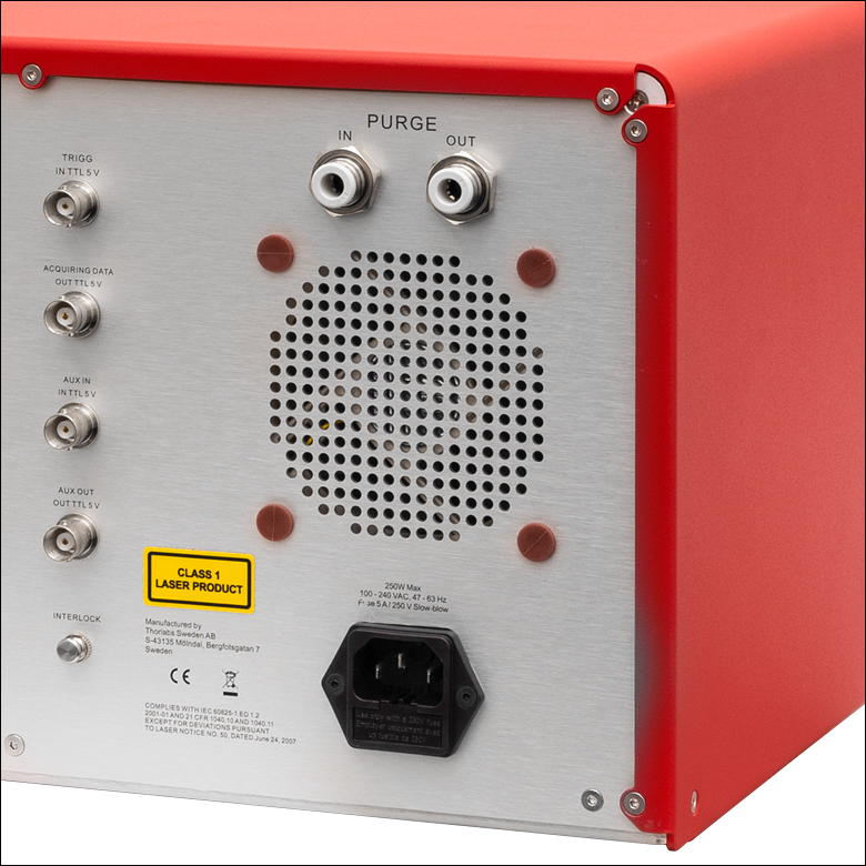
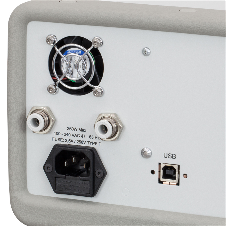
To reduce the presence of water absorption lines in the MIR region of the spectrum, our OSAs feature two quick-connect hose connections (1/4" ID) on the back panel, through which the interferometer can be purged with dry air or nitrogen. Our Pure Air Circulator Unit, which uses hosing that can be directly inserted into these connectors, is ideal for this task.
Resolution and Sensitivity
The resolution of this type of instrument depends on the optical path difference (OPD) between the two paths in the interferometer. It is usually easier to understand the resolution in terms of wavenumbers (inverse centimeters), as opposed to wavelength (nanometers) or frequency (terahertz).
Assume we have two narrowband sources, such as lasers, with a 1 cm-1 energy difference, 6500 cm-1 and 6501 cm-1. To distinguish between these signals in the interferogram, we would need to move away 1 cm from the point of zero path difference (ZPD). The OSA20xC can move ±4 cm in OPD and thus spectral features 0.25 cm-1 apart can be resolved, while the Redstone OSA30x can move 16 cm in OPD and resolve spectral features that are 0.063 cm-1 apart. The resolution of the instrument can be calculated as:
![]()
where Δλ is the resolution in pm, Δk is the resolution in cm-1, and λ is the wavelength in µm. The resolution in pm as a function of wavelength, converted using this formula, is shown in Figure 1.3.
The resolution of the OSA20xC instruments can be set to High or Low in the main window of the software. In high resolution mode, the retroreflectors translate by the maximum of ±1 cm (±4 cm in OPD), while in low resolution mode, the retroreflectors translate by ±0.25 cm (±1 cm in OPD). The Redstone OSA30x instruments can be set to one of four resolution modes: High, Medium High, Medium Low, or Low. These settings correspond to OPDs of 16 cm, 4 cm, 1 cm, and 2.5 mm, respectively. The OSA software can cut the length of the interferogram that is used in the calculation of the spectrum in order to remove spectral contributions from high-frequency components.
The sensitivity of the instrument depends on the electronic gain used in the sensor electronics. Since an increased gain setting reduces the bandwidth of the detectors, the instrument will run slower when higher gain settings are used. Figures 1.4 and 1.5 show the dependency of the noise floor on the wavelength and OSA model.
Click to Enlarge
Figure 1.4 Noise Floor in Absolute Power Mode
Absolute Power mode is recommended for narrowband sources. The OSA203C noise floor was measured in low-temperature mode.
Click to Enlarge
Figure 1.5 Noise Floor in Power Density Mode
Power Density mode is recommended for broadband sources. The OSA203C noise floor was measured in low-temperature mode.
Absolute Power and Power Density
The vertical axis of the spectrum can be displayed as Absolute Power (Figure 1.4) or Power Density (Figure 5), both of which can be displayed in either a linear or logarithmic scale. In Absolute Power mode, the total power displayed is based on the actual instrument resolution for that specific wavelength; this setting is recommended to be used only with narrow spectrum input light. For broadband devices, it is recommended that the Power Density mode is used. Here the vertical axis is displayed in units of power per unit wavelength, where the unit wavelength is based upon a fixed wavelength band and is independent of the resolution setting of the instrument.
Interferogram Data Acquisition
For the OSA20xC models, the interference pattern of the reference laser is used to clock a 16-bit analog-to-digital converter (ADC) such that samples are taken at a fixed, equidistant optical path length interval. The HeNe reference fringe period is digitized and its frequency multiplied by a phase-locked loop (PLL), leading to an extremely fine sampling resolution. Multiple PLL filters enable frequency multiplication settings of 16X, 32X, 64X, or 128X. At the 128X multiplier setting, data points are acquired approximately every 1 nm of carriage travel. The multiple PLL filters enable the user to balance the system parameters of resolution and sensitivity against the acquisition time and refresh rate.
The Redstone OSA30x instruments instead sample the interferogram at a fixed frequency of up to 1 MHz with an 18-bit ADC while the retroreflector platform moves at a constant speed controlled by a PID loop. At the highest sensitivity setting, there is one data point collected about every 1 nm of travel. The collected data is resampled to fit up to 128 data points per reference laser period.
The fine sampling can be very useful when the measured light is weak and broadband, causing only a very short interval in the interferogram at the ZPD to contain all the spectral information. This portion of the interferogram is normally referred to as the center burst.
A high-speed USB link transfers the interferograms to the OSA software, which is highly optimized to take full advantage of modern multi-core processors, as well as top-performing graphics processing units (GPUs). The software performs a number of calculations to analyze and condition the input waveform in order to obtain the highest possible resolution and signal-to-noise ratio (SNR) at the output of the Fast Fourier transform (FFT).
The OSA20xC devices make use of a very low noise and low distortion detector amplifier with automatic gain control provides a large dynamic range, allows optimal use of the ADC, and ensures excellent signal-to-noise (SNR) for up to 10 mW of input power. For low-power signals, the system can typically detect less than 100 pW from narrowband sources. The balanced detection architecture enhances the SNR of the system by enabling the OSA20xC to use all of the light that enters the interferometer, while also rejecting common mode noise.
The Redstone OSA detector modules contain high gain-bandwidth product (GBP) amplifiers, which fully exploit the detectors’ dynamic range, combined with high-current low-noise buffers driving a high-bandwidth 18-bit ADC. Automatic amplifier adjustments optimize the number of used ADC bits (filling ratio). Switchable optical attenuators provide for a wide input power range even with early saturating IR-detectors. Differential amplifiers, as well as balanced transmission architectures with effective screening and filtering techniques, assure a good signal integrity for a high spurious-free dynamic range.

Click to Enlarge
Figure 1.6 A Typical Interferogram
Interferogram Data Processing
The interferograms (see Figure 1.6) generated by the instrument vary from 50 thousand to 16 million data points depending on the resolution and sensitivity mode settings employed. The FT-OSA software analyzes the input data and intelligently selects the optimal FFT algorithm from our internal library.
Additional software performance is realized by utilizing an asynchronous, multi-threaded approach to collecting and handling interferogram data through the multitude of processing stages required to yield spectrum information. The software's multi-threaded architecture manages several operational tasks in parallel by actively adapting to the PC's capabilities, thus ensuring maximum processor bandwidth utilization. Each of our FT-OSA instruments ships complete with a laptop computer that has been carefully selected to ensure that both the data processing and user interface operate optimally.
Wavelength Meter Mode
When narrowband optical signals are analyzed, the FT-OSA automatically calculates the center wavelength of the input, which can be displayed in a window just below the main display that presents the overall spectrum. The central wavelength, λ, is calculated by counting interference fringes (periods in the interferogram) from both the input and reference lasers according to the following formula:

Here, mref is the number of fringes for the reference laser, mmeas is the number of fringes from the input laser, nref is the index of refraction of air at the reference laser wavelength (632.9918 nm or 1532.8323 nm), and λref,vac is the vacuum wavelength of the reference laser. nmeas is the index of refraction of air at the wavelength λmeas,vac and is determined iteratively from λmeas,air (that is, the measured wavelength in air) using a modified version of the Edlén formula (OSA software version 2.90 or lower) or Ciddor's formula (OSA software version 3.0 and higher).
The resolution of the FT-OSA operating as a wavelength meter is substantially higher than the system when it operates as a broadband spectrometer because the system can resolve a fraction of a fringe (see the Interferogram Data Acquisition section above). In practice, the resolution of the system is limited by the bandwidth and structure of the unknown input, noise in the detectors, drift in the reference laser, interferometer alignment, and other systematic errors. In Wavelength Meter mode, the system has been found to offer reliable results as low as ±0.1 pm in the visible spectrum and ±0.2 pm in the NIR/IR (see the Specs tab on the main OSA presentation for details).
The software evaluates the spectrum of the unknown input in order to determine an appropriate display resolution. If the data is unreliable, as would be the case for a multiple peak spectrum, the software disables the Wavelength Meter mode so it does not provide misleading results.
Wavelength Calibration and Accuracy
The OSA20xC instruments use a built-in stabilized HeNe reference laser with a vacuum wavelength of 632.9918 nm. The use of a stabilized HeNe ensures long-term wavelength accuracy as the dynamics of the stabilized HeNe are well-known and controlled. The Redstone OSA30x models incorporate a frequency-locked reference laser with a vacuum wavelength of 1532.8323 nm. Because of the frequency-lock, long-term wavelength accuracy is ensured, and the reference laser is connected to an FC/APC output and can be fed into the instrument fiber input for additional calibration if so desired.
The instrument is factory-aligned so that the reference and unknown input beams experience the same optical path length change as the interferometer is scanned. The effect of any residual alignment error on wavelength measurements is less than 0.5 ppm; the input beam pointing accuracy is ensured by a high-precision ceramic receptacle and a robust interferometer cavity design. No optical fibers are used within the scanning interferometer. The wavelength of the reference laser in air is actively calculated for each measurement using the Edlén formula (OSA software version 2.90 or lower) or Ciddor's formula (OSA software version 3.0 and higher) with temperature and pressure data collected by sensors internal to the instrument.
| Table 1.7 Optical Rejection Ratio | ||
|---|---|---|
| Distance from 1532 nm Peak | OSA205C | OSA305 |
| 0.2 nm (25 GHz) | 30 dB | 40 dB |
| 0.8 nm (100 GHz) | 37 dB | 42 dB |
| 6.2 nm (800 GHz) | 44 dB | 45 dB |
| 7.8 nm (1000 GHz) | 44 dB | 45 dB |
Optical Rejection Ratio
The ability to measure low-level signals close to a peak is determined by the optical rejection ratio (ORR) of the instrument. It can be seen as the filter response of the OSA, and can be defined as the ratio between the power at a given distance from the peak and the power at the peak.
If the ORR is not higher than the optical signal-to-noise ratio of the source to be tested, the measurement will be limited by the OSA's response, rather than reflecting a true property of the tested source. Table 1.7 provides an example.
Software Tutorial Videos
To help customers learn about, use, and understand the Optical Spectrum Analyzer software, we have prepared several short narrated videos that describe the basic aspects of the software and the optimal settings for common types of measurements. Although the OSA model shown in the videos has been discontinued, the principles of operation have not changed.
Basic Features of OSA SoftwareTopics Covered
Length: 4:41 |
Tips for Choosing the Best Acquisition SettingsTopics Covered
Length: 3:54 |
Measuring a Narrowband SourceTopics Covered
Length: 3:13 |
Measuring Optical Input PowerTopics Covered
Length: 1:24 |
Performing a Filter MeasurementTopics Covered
Length: 2:38 |
Analyzing Pulsed Sources Using the OSA20xC and Redstone® Instruments
Introduction and Summary of Results
While Thorlabs' Optical Spectrum Analyzers (OSAs) have been designed for analysis of CW signals, it is possible to measure pulsed spectra under certain situations. Measurement of pulsed spectra suffers from several issues that must be overcome for accurate measurements; for instance, "spectral ghosts" arise due to the pulsed nature of the source as well as the varying optical path difference (OPD) of the OSA. In addition, the noise floor for pulsed sources is much higher than that for CW sources. One method for measuring pulsed sources with the OSA involves taking several successive measurements at the different sensitivity levels; the minimum at each wavelength of these traces is used to form a combined spectrum, which suppresses the spectral ghosts. This technique is implemented in the OSA software by choosing "Pulsed" under the "Sweep" or "Instrument" menu. The following tutorial explains the rationale of this technique and the pulsed sources for which it is useful.
In summary, for pulse rates over 30 kHz for the OSA20xC and 6 kHz for the OSA30x, standard measurements can be performed because the repetition rate is greater than the detectors' bandwidth. For broadband signals with low repetition rates, care must be taken to ensure that the "zero burst" of the interferogram coincides with one of the pulses. Also, when using a pulsed source "Automatic Gain" does not work properly, so the user must monitor the interferogram and manually set the gain and offset so that a strong, but not saturated, signal is obtained. For more information on using a pulsed source with our OSA instruments, please contact Tech Support.
Impact of a Pulsed Source on the Interferogram and Spectrum
As the Optical Path Difference (OPD) continuously changes during an interferogram measurement, a pulsed light source effectively modulates the interferogram. In the case of 100% modulation (i.e. on-off pulsation), the resulting interferogram will contain repetitive regions (slots) with no information. These slots correspond to OPDs when no light can be measured by the detector assembly. The resulting interferogram in this case is the true interferogram masked with the pulsed signal. Figure 3.1 shows measured interferograms and the corresponding spectra for a light source in CW and pulsed operation. Although the spectrum of the light source is expected to be the same for CW and pulsed operation (ignoring small changes in the peak shape and position due to, for example, a decreased LD chip temperature resulting from the pulsed drive), additional frequency artifacts appear symmetrically about the expected peak due to the modulation in the pulsed interferogram. These "spectral ghosts" are a result of the temporal, rather than the spectral, behavior of the source. To measure the true spectrum of the light source, it is crucial to make the spectral ghosts sufficiently small or force the spectral ghosts to fall outside the frequency / wavelength range of interest.
Figure 3.1 Interferograms and spectra for a narrowband light source in CW (Top) and pulsed at 20 kHz (Bottom)
operation measured with an OSA20xC device. The square wave modulation of the interferogram induces the spectral ghosts shown in the bottom right plot.

Click to Enlarge
Figure 3.2 Stacked spectra for 55 pulse repetition rates between 100 Hz and 100 kHz for a 1550 nm DFB laser diode measured with an OSA20xC device. The intensity is mapped in a logarithmic scale. OSA settings: High Resolution, High Sensitivity, No Apodization, 5 averages.
Mathematically, the resultant spectrum of a pulsed source can be described by a convolution between the spectrum of the light source and the spectrum corresponding to the pulses. As a result, the impact of these artifacts will vary with the pulse repetition rate and the modulation depth of the light source as well as the OPD sample rate (cm/s) of the OSA. The modulation depth of the light source determines the amplitude of the spectral ghosts; a weak modulation yields weak spectral ghosts while a modulation of 100% (on-off pulsation) yields the strongest spectral ghosts.
Figure 3.2 shows how the behavior of the spectral ghosts as a function of the pulse repetition rate for a narrowband source. In the figure, the spectra were measured for 55 pulse repetition rates between 100 Hz and 100 kHz for a 1550 nm DFB laser diode connected to an OSA20xC device. We have offset the y-axis such that the true peak (the light gray horizontal line) has been centered at a relative frequency of 0 THz. Figure 3.2 can be divided into three regions: fp ≤ 3 kHz, 3 kHz < fp ≤ 30 kHz and fp >30 kHz. For fp ≤ 3 kHz, the spectral ghosts are clearly observed symmetrically about the true peak within the resultant spectrum, and move farther and farther away from the true peak as the repetition rate increases. The second region starts above 3 kHz, when the first spectral ghosts have moved beyond the spectral range of the OSA. However, aliasing / folding create higher order spectral ghosts that appear within the spectral range of the OSA. In the third region, fp > 30 kHz, the resulting spectrum agrees very well with the CW spectrum because the repetition rate of the source has extended beyond the bandwidth limit of the detectors. As a result, the pulsed source appears like a CW source to the OSA electronics.
"Pulsed Mode" Operation
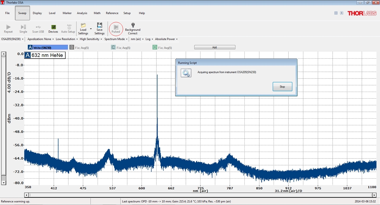
To help remove some of these frequency artifacts, the OSA software contains a "Pulsed Mode" measurement (Figure 3.3). The "slot period" of the interferogram, determined by the pulse repetition rate of the light source and the OPD rate of the OSA, affects the positions of the spectral ghosts. A shorter slot period yields a larger spectral distance between the true peak and the first order ghost peaks. In Thorlabs' OSAs, the OPD sample rate is given by the speed of the moving carriage which can be controlled by the user indirectly through the sensitivity setting. The higher the sensitivity setting is, the slower the speed of the moving carriage will be. Thus, the use of the "High" sensitivity mode of the OSA will provide the shortest slot period (i.e. the largest spacing between the feature of interest and the frequency artifacts). In Pulsed Mode, the software acquires several spectra with different sensitivity settings (or OPD sample rates) and filters out the changing spectral features. The sensitivity is set to increasingly high levels, starting with Low. After reaching the highest sensitivity, it is again set to Low, yielding a periodically changing sensitivity. The captured spectra are then combined using the minimum hold function. The spectral ghosts (Figure 3.4), whose positions depend on the sensitivity setting (the OPD rate), can then be reduced in the measurement as shown in Figure 3.4. It is important to note that the Pulse Mode button is found under the "Sweep" or "Instrument" menu and can be started only after the current sweep has been completely stopped.
Click to Enlarge
Figure 3.3 Screenshot of the OSA software in Pulsed
Mode; the icon is indicated with a red circle.

Click to Enlarge
Figure 3.4 (Left) Measured spectra for a narrowband light source pulsed at 1 kHz with (from top to bottom) Low, Medium-Low, Medium-High, and High sensitivity settings (i.e. a decreasing OPD sample rate from top to bottom). (Right) Measured spectrum using the Pulsed Mode, i.e., a minimum hold combination of spectra similar to those shown in the bottom left plots.
Narrowband Light Source
A DFB laser diode emitting at 1550 nm (193.7 THz) was used as a narrowband light source and measured with an OSA203C in both CW and pulsed operation. The laser diode was modulated (using Thorlabs' ITC4001 controller) with repetition rates between fp = 20 Hz and 100 kHz. Five averaged spectra were captured for each light source setting; the CW spectra were acquired in high sensitivity mode, and the pulsed spectra were recorded in both high sensitivity and pulsed mode. It is important to note that the pulsed mode does not allow averaging. Instead the minimum hold function was used for 5 sets of spectra from the four different sensitivity settings.
Figure 3.5 shows the resultant spectra for the source in CW mode as well as four different pulse repetition rates between 100 Hz and 100 kHz. As the pulse rate increases, the spectral ghosts (as recorded in the high sensitivity mode) move further and further away from the true laser peak until nearly identical spectra are obtained at 100 kHz.
Figure 3.5 Spectra from measurements of a 1550 nm (193.7 THz) pulsed narrowband source. Pulse repetition rates shown (left to right): 100 Hz, 1 kHz, 13 kHz, and 100 kHz. Black line: CW measurement; blue line: pulsed source measured with high sensitivity; red line: pulsed source measured using the pulsed mode. The lower plots are the same data set as the upper plots only on a shorter frequency scale.
Broadband Light Source
A gain chip was driven in amplified spontaneous emission (ASE) mode to create a broadband light source centered at 850 nm (352.9 THz) with a FWHM of 36.4 nm (15.2 THz). An OSA201C was used to measure the spectrum for CW and pulsed operation with pulse repetition rates from fp = 100 Hz to 100 kHz. The ASE diode was modulated (using Thorlabs' ITC4001 controller) with a 50% duty cycle square wave. A total of 10 averaged spectra were acquired using high sensitivity (CW and pulsed sources) and the pulsed mode (pulsed source). Because pulsed mode does not allow averaging, the minimum hold function was used to acquire five sets of the four different sensitivity settings.
In general, the spectral ghosts are less visible for the broadband peak compared to a narrowband peak. However, the noise floor is higher and the spectral ghosts are clearly seen for a repetition rate of 1 kHz and 13 kHz in Figure 3.6. Similar to the narrowband source, the spectral ghosts move farther and farther away from the true peak with increasing repetition rate. For a repetition rate of 100 kHz both the measurement using high sensitivity and pulsed mode agree well with the CW measurement. As seen, the shape of the peak is slightly different for the CW spectrum compared to the pulsed spectrum. This is not related to the behavior of the OSA but due to a true change in the peak during pulsed operation, e.g., a lower chip temperature.
Figure 3.6 Measured spectra from a pulsed broadband source with a center wavelength (frequency) of 850 nm (352.9 THz). The pulse repetition rates shown are 100 Hz, 1 kHz, 13 kHz, and 100 kHz. Top and bottom rows show the full spectrum and the ±50 THz range surrounding the peak, respectively. Black line: CW; blue line: pulsed source measured using high sensitivity; red line: Pulsed Mode.
It is extremely important to note that in general, one has to be careful when measuring broadband peaks at low repetition rates. Since most of the information in the interferogram is located about the zero burst, the peak can be completely missed if the zero burst coincides with no light falling on the detector as shown in Figure 3.7.
Figure 3.7 Measured interferograms (left) and spectra (right) obtained when the zero burst resulting from a broadband
source coincides with a pulse (blue curves) and is missed if no light reaches the detector at OPD ~ 0 (red curves).
Click to Enlarge
Figure 3.8 (Top) Central portion of a captured interferogram from a broadband femtosecond laser. (Bottom) Measured spectrum captured using an OSA201 (red line) and a measured reference spectrum captured using a scanning grating-based OSA (blue line).
Femtosecond Pulsed Laser
We measured the spectrum of a broadband femtosecond laser using an OSA201C. This laser has a repetition rate of 85 MHz, a pulse width of 10 fs, and an average power of about 300 µW into the fiber. The OSA was set to Low Resolution, High Sensitivity, 5 spectral averages, and no apodization. Light output from the laser was collected with a fiber patch cable (SM600 fiber; 0.12 NA, 4.6 µm mode field diameter at 680 nm) connected to the OSA.
Figure 3.8 shows the interferogram collected during acquisition, which does not contain any empty slots. This was expected as the 85 MHz repetition rate of the laser is well beyond the 40 kHz bandwidth of the OSA's detectors. Furthermore, the spectrum measured by the OSA agrees very well with the reference spectrum captured using a grating-based OSA that is scanned slowly enough to provide adequate signal for each wavelength measured.
| Table 4.3 Specifications | ||
|---|---|---|
| Item # | Frequency Range | Level Sensitivity (Click for Graph)a |
| OSA207C | 833 - 10 000 cm-1 (12.0 - 1.0 µm) |
 Absolute Power  Power Density |
| OSA205C | 1786 - 10 000 cm-1 (5.6 - 1.0 µm) |
|
| OSA305 | ||
| OSA203C | 3846 - 10 000 cm-1 (2.6 - 1.0 µm) |
|
| OSA302 | 4000 - 40 000 cm-1 (2.5 µm - 250 nm) |
|
Click to Enlarge
Figure 4.2 Rear-Mounted Hose Connections for Purging the Redstone® OSA30x Cavity
Click to Enlarge
Figure 4.1 Hose Connections for Purging OSA20xC Cavity
Gas Detection and Identification Using an Optical Spectrum Analyzer
As shown in Table 4.3, many of Thorlabs' Optical Spectrum Analyzers (OSAs) offer detection extending into the mid-infrared (MIR) region of the spectrum, where many gaseous species characteristically absorb. Moreover, the software included with all OSA models supports files from the HITRAN database, a spectroscopic reference standard. These files can be fit to measured traces to identify unknown gases. With the ability to fit multiple analytes simultaneously and built-in hose connections (compatible with Thorlabs' Pure Air Circulator Unit) for purging the interferometer's cavity of trace gases, these OSAs are ideal for use in home-built gas detection setups.
Experimental Setup
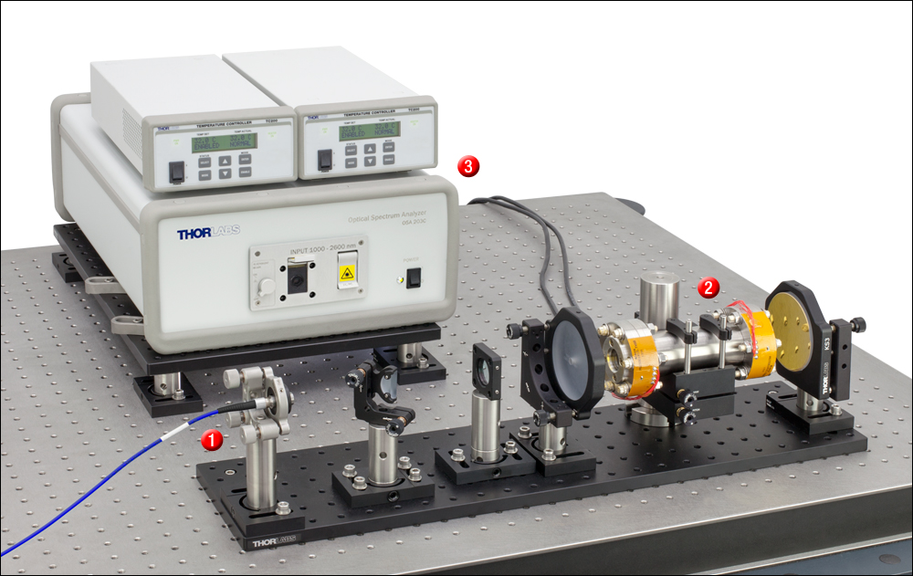
A sample detection setup is shown in Figure 4.4. Broadband MIR light generated by a Stabilized Light Source is emitted from a zirconium fluoride fiber ( ), collimated, then sent into a multipass cell (
 ) containing the gas analyte in a sample chamber. Each end of the chamber is sealed by an airtight, transparent window. Gold mirrors on each side of the chamber provide multiple reflections that increase the sensitivity of the measurement; the mirror closer to the light source has a center hole to allow the optical path to enter and exit the chamber. Light exiting the detection setup is collimated by a long-focal-length lens and reflected by a D-shaped mirror into the free-space port of the OSA203C (
 ). The temperature inside the chamber is elevated and held constant in order to prevent the gas's absorption lines from shifting during the measurement.
Click to Enlarge
Figure 4.4 A gas detection setup using the OSA203C. A multipass cell is constructed around the sample chamber (
) in order to provide high detection sensitivity for the gaseous species sealed inside.| Parts Used in Sample Setup (Click Here for a Metric Item List) |
||
|---|---|---|
| Item # | Qty. | Description |
Light Source  |
||
| SLS202La | 1 | Stabilized Fiber-Coupled Light Source, 450 nm - 5.5 µm (Not Shown) |
| FB2000-500 | 1 | Ø1" Bandpass Filter, 2.0 µm CWL, 0.5 µm FWHM (Not Shown) |
| MZ21L1 | 1 | ZrF4 Multimode Fiber Patch Cable, SMA905 Connectors |
| F028SMA-2000 | 1 | SMA905 Fiber Collimator, AR Coated: 1.8 - 3.0 µm |
| POLARIS-K1b | 1 | Polaris® Ø1" Kinematic Mirror Mount |
| AD11NT | 1 | Unthreaded Adapter for Ø11 mm Cylindrical Components |
Detection  |
||
| OSA203C | 1 | Optical Spectrum Analyzer, 1.0 - 2.6 µm |
| TC200c | 2 | Temperature Controller |
| MB1218 | 1 | 12" x 18" Aluminum Breadboard |
| CF125C | 3 | Clamping Fork with Captive Screw |
| Other Optomechanics | ||
| RS2 | 6 | Ø1" Pillar Post, Length = 2" |
| RS3 | 1 | Ø1" Pillar Post, Length = 3" |
| RS4 | 2 | Ø1" Pillar Post, Length = 4" |
| BA2F | 9 | Flexure Clamping Base |
| Parts Used in Sample Setup (Continued) (Click Here for a Metric Item List) |
||
|---|---|---|
| Item # | Qty. | Description |
Beam Path Into and Out of Multipass Cell  |
||
| LB4374 | 1 | Uncoated, Ø1", f = 1000 mm Bi-Convex UV Fused Silica Lens |
| CP33 | 1 | Post-Mountable, SM1-Threaded Cage Plate for Ø1" Optics |
| CM750-200-M01 | 2 | Ø75 mm, f = 200 mm Protected Gold Concave Mirror (One Mirror Contains a Center Hole, Similar to Our Herriott Cell Mirrors) |
| KS3 | 2 | Kinematic Mount for Ø3" Mirrors |
| VPCH512 | 2 | Ø2.75" CF Flange with CaF2 Window, 180 nm - 8.0 µm |
| N/A | 1 | Sample Chamber |
| C1513 | 1 | Kinematic V-Clamp Mount |
| PM4 | 2 | Clamping Arm (One Clamping Arm is Included with Each C1513 Mount) |
| P6 | 1 | Ø1.5" Mounting Post, Length = 6" |
| PB2 | 1 | Base for Ø1.5" Mounting Posts |
| PFD10-03-M01 | 1 | 1" Protected Gold D-Shaped Pickoff Mirror |
| KM100D | 1 | Kinematic Mount for 1" D-Shaped Pickoff Mirrors |
| MB624 | 1 | 6" x 24" Aluminum Breadboard |
Assigning Peaks in an Unknown Spectrum
Once the experimental spectrum is obtained, the user chooses a gas or gas mixture that is believed to be present inside the sample chamber, as shown in Figure 4.5. There is no limit to how many species can be considered in the fit, but the fit is more likely to converge when fewer species are chosen. The OSA software ships with HITRAN line-by-line references for acetylene (C2H2), water vapor (H2O), and carbon dioxide (CO2), and can import additional references downloaded from the HITRAN database. Previously saved spectra in the OSA file format can also be used as references. See the References section of the ThorSpectra manual for details.
The user may optionally allow the software to shift the reference spectrum in wavelength in order to account for measurement effects related to the sample environment. In the case of gas mixtures (i.e., fits performed using more than one reference spectrum), the software scales the intensity of each reference as needed to reproduce the measured spectrum. As shown in Figure 4.6, the output of the fit operation is a graph comparing the measured spectrum, each scaled (and possibly also shifted) reference spectrum, and the sum of the scaled reference spectra.

Click to Enlarge
Figure 4.5 In the Reference Fit Setup tab, checkboxes are used to indicate which gaseous species to consider in the fit. The absorption lines can be either "fixed" or "free"; the latter allows the software to shift the reference spectrum in wavelength. The measurement conditions for the HITRAN references are also displayed.
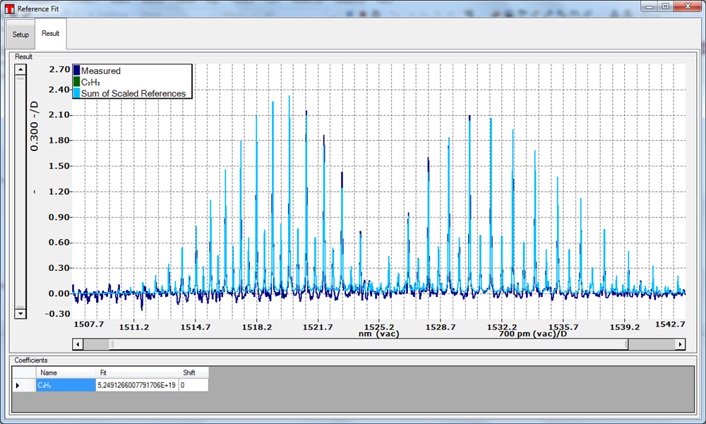
Click to Enlarge
Figure 4.6 In the Reference Fit Result tab, the fitted spectrum is displayed simultaneously with the measured spectrum. The fitted spectrum is the sum of the scaled reference spectra included in the fit. The scaled spectrum for each individual gaseous species is also shown.
| Posted Comments: | |
| No Comments Posted |