 Products Home
Laser Scanning Microscopy Tutorial

Please Wait

Laser Scanning Microscopy TutorialLaser scanning microscopy (LSM) is an indispensable imaging tool in the biological sciences. In this tutorial, we will be discussing confocal fluorescence imaging, multiphoton excitation fluorescence imaging, and second and third harmonic generation imaging techniques. We will limit our discussions to point scanning of biological samples with a focus on the technology behind the imaging tools offered by Thorlabs. |
Introduction
The goal of any microscope is to generate high-contrast, high-resolution images. In much the same way that a telescope allows scientists to discern the finest details of the universe, a microscope allows us to observe biological functioning at the nanometer scale. Modern laser scanning microscopes are capable of generating multidimensional data (X, Y, Z, τ, λ), leading to a plethora of high-resolution imaging capabilities that further the understanding of underlying biological processes.
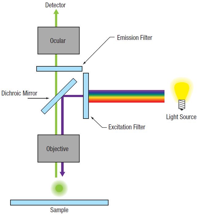
In conventional widefield microscopy (Figure 72A), high-quality images can only be obtained when using thin specimens (on the order of one to two cell layers thick). However, many applications require imaging of thick samples, where volume datasets or selection of data from within a specific focal plane is desired. Conventional widefield microscopes are unable to address these needs.
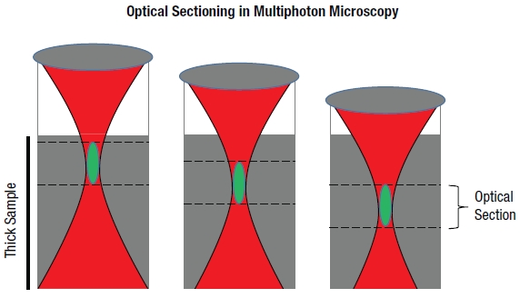
LSM, in particular confocal LSM and multiphoton LSM, allows for the visualization of thin planes from within a thick bulk sample, a technique known as optical sectioning. In confocal LSM, signals generated by the sample outside of the optical focus are physically blocked by an aperture, preventing their detection. Multiphoton LSM, as we will discuss later, does not generate any appreciable signal outside of the focal plane. By combining optical sectioning with incremented changes in focus (Figure 72B), laser scanning microscopy techniques can recreate 3D representations of thick specimen.
|
Figure 72A Widefield Epi-Fluorescence
|
|
Figure 72B Optical Sections (Visualization of Thin Planes within a Bulk Sample)
Signal generated by the sample is shown in green. Optical sections are formed by discretely measuring the signal generated within a specific focal plane. In confocal LSM, out-of-focus light is rejected through the use of a pinhole aperture, thereby leading to higher resolution. In multiphoton LSM, signal is only generated in the focal volume. Signal collected at each optical section can be reconstructed to create a 3D image. |

Contrast Mechanisms in LSM
Biological samples typically do not have very good contrast, which leads to difficulty in observing the boundaries between adjacent structures. A common method for improving contrast in laser scanning microscopes is through the use of fluorescence.
In fluorescence, a light-emitting molecule is used to distinguish the constituent of interest from the background or neighboring structure. This molecule can already exist within the specimen (endogenous or auto-fluorescence), be applied externally and attached to the constituent (chemically or through antibody binding), or transfected (fluorescent proteins) into the cell.
In order for the molecule to emit light (fluoresce) it must first absorb light (a photon) with the appropriate amount of energy to promote the molecule from the ground state to the excited state, as seen in Figure 72C (a). Light is emitted when the molecule returns back down to the ground state. The amount of fluorescence is proportional to the intensity (I) of the incident laser, and so confocal LSM is often referred to as a linear imaging technique. Natural losses within this relaxation process require that the emitted photon have lower energy—that is, a longer wavelength—than the absorbed photon.
Multiphoton excitation [Figure 72C (b)] of the molecule occurs when two (or more) photons, whose sum energy satisfies the transition energy, arrive simultaneously. Consequently, the two arriving photons will be of lower energy than the emitted fluorescence photon.
There are also multiphoton contrast mechanisms, such as harmonic generation and sum frequency generation, that use non-absorptive processes. Under conditions in which harmonic generation is allowed, the incident photons are simultaneously annihilated and a new photon of the summed energy is created, as illustrated in Figure 72C (c).
Further constituent discrimination can be obtained by observing the physical order of the harmonic generation. In the case of second harmonic generation (SHG), signal is only generated in constituents that are highly ordered and lacking inversion symmetry. Third harmonic generation (THG) is observed at boundary interfaces where there is a refractive index change. Two-photon excitation and SHG are nonlinear processes and the signal generated is dependent on the square of the intensity (I2).
The nonlinear nature of signal generation in multiphoton microscopy means that high photon densities are required to observe SHG and THG. In order to accomplish this while maintaining relatively low average power on the sample, mode-locked femtosecond pulsed lasers, particularly Ti:Sapphire lasers, have become the standard.
Another consideration to be made in nonlinear microscopy is the excitation wavelength for a particular fluorophore. One might think that the ideal excitation wavelength is twice that of the one-photon absorption peak. However, for most fluorophores, the excited state selection rules are different for one- and two-photon absorption.
This leads to two-photon absorption spectra that are quite different from their one-photon counterparts. Two-photon absorption spectra are often significantly broader (can be >100 nm) and do not follow smooth semi-Gaussian curves. The broad two-photon absorption spectrum of many fluorophores facilitates excitation of several fluorescent molecules with a single laser, allowing the observation of several constituents of interest simultaneously.
All of the fluorophores being excited do not have to have the same excitation peak, but should overlap each other and have a common excitation range. Multiple fluorophore excitation is typically accomplished by choosing a compromising wavelength that excites all fluorophores with acceptable levels of efficiency.
|
Figure 72C Signal Generation in Laser Scanning Microscopy
Absorptive Process (a, b): The absorption of one or more excitation photons (λEX) promotes the molecule from the ground state (S0) to the excited state (S1). Fluorescence (λEM) is emitted when the molecule returns to the ground state. Non-Absorptive Process (c): The excitation photons (λEX) simultaneously convert into a single photon (λSHG,THG) of the sum energy and half (for SHG) or one-third (for THG) the wavelength.
|
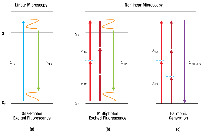

Image Formation
In a point-scanning LSM, the single-plane image is created by a point illumination source imaged to a diffraction-limited spot at the sample, which is then imaged to a point detector. Two-dimensional en face images are created by scanning the diffraction-limited spot across the specimen, point by point, to form a line, then line by line in a raster fashion.
The illuminated volume emits a signal which is imaged to a single-element detector. The most common single-element detector used is a photomultiplier tube (PMT), although in certain cases, avalanche photodiodes (APDs) can be used. CCD cameras are not typically used in point-scanning microscopes, though are the detector of choice in multifocal (i.e. spinning disk confocal) applications.
The signal from the detector is then passed to a computer which constructs a two-dimensional image as an array of intensities for each spot scanned across the sample. Because no true image is formed, LSM is referred to as a digital imaging technique. A clear advantage of single-point scanning and single-point detection is that the displayed image resolution, optical resolution, and scan field can be set to match a particular experimental requirement and are not predefined by the imaging optics of the system.
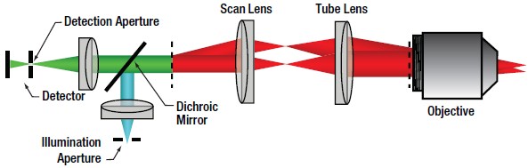
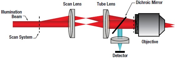
| Figure 72D Confocal Optical Path
|
Confocal LSM
In confocal LSM, point illumination, typically from a single mode, optical-fiber-coupled CW laser, is the critical feature that allows optical sectioning. The light emitted from the core of the single mode optical fiber is collimated and used as the illumination beam for scanning. The scan system is then imaged to the back aperture of the objective lens which focuses the scanned beam to a diffraction-limited spot on the sample. The signal generated by the focused illumination beam is collected back through the objective and passed through the scan system.
After the scan system, the signal is separated from the illumination beam by a dichroic mirror and brought to a focus. The confocal pinhole is located at this focus. In this configuration, signals that are generated above or below the focal plane are blocked from passing through the pinhole, creating the optically sectioned image (Figure 72B). The detector is placed after the confocal pinhole, as illustrated in Figure 72D. It can be inferred that the size of the pinhole has direct consequences on the imaging capabilities (particularly, contrast, resolution and optical section thickness) of the confocal microscope.
The lateral resolution of a confocal microscope is determined by the ability of the system to create a diffraction-limited spot at the sample. Forming a diffraction-limited spot depends on the quality of the laser beam as well as that of the scan optics and objective lens.
The beam quality is typically ensured by using a single mode optical fiber to deliver the excitation laser light as a Gaussian point source, which is then collimated and focused into a diffraction-limited beam. In an aberration-free imaging system, obtained by using the highest quality optical elements, the size of this focus spot, assuming uniform illumination, is a function of excitation wavelength (λEX) and numerical aperture (NA) of the objective lens, as seen in Equation 1.
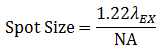
Equation 1 Spot Size
In actuality, the beam isn't focused to a true point, but rather to a bullseye-like shape. The spot size is the distance between the zeros of the Airy disk (diameter across the middle of the first ring around the center of the bullseye) and is termed one Airy Unit (AU). This will become important again later when we discuss pinhole sizes.
The lateral resolution of the imaging system is defined as the minimum distance between two points for them to be observed as two distinct entities. In confocal (and multiphoton) LSM, it is common and experimentally convenient to define the lateral resolution according to the full width at half maximum (FWHM) of the individual points that are observed.
Using the FWHM definition, in confocal LSM, the lateral resolution (Rlateral,confocal) is:
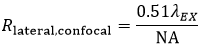
Equation 2 Lateral Resolution, Confocal LSM
and the axial resolution (Raxial,confocal) is:
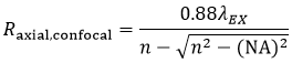
Equation 3 Axial Resolution, Confocal LSM
where n is the refractive index of the immersion medium.
It is interesting to note that in a confocal microscope, the lateral resolution is solely determined by the excitation wavelength. This is in contrast to widefield microscopy, where lateral resolution is determined only by emission wavelength.
To determine the appropriate size of the confocal pinhole, we multiply the excitation spot size by the total magnification of the microscope:

Equation 4 Pinhole Diameter
As an example, the appropriate size pinhole for a 60X objective with NA = 1.0 for λEX = 488 nm (Mscan head = 1.07 for the Thorlabs Confocal Scan Head) would be 38.2 μm and is termed a pinhole of 1 AU diameter. If we used the same objective parameters but changed the magnification to 40X, the appropriate pinhole size would be 25.5 μm and would also be termed a pinhole of 1 AU diameter. Therefore, defining a pinhole diameter in terms of AU is a means of normalizing pinhole diameter, even though one would have to change the pinhole selection for the two different objectives.
Theoretically, the total resolution of a confocal microscope is a function of the excitation illumination spot size and the detection pinhole size. This means that the resolution of the optical system can be improved by reducing the size of the pinhole. Practically speaking, as we restrict the pinhole diameter, we improve resolution and confocality, but we also reduce the amount of signal reaching the detector. A pinhole of 1 AU is a good balance between signal strength, resolution, and confocality.
| Figure 72E Multiphoton Optical Path
|
Multiphoton LSM
In multiphoton LSM, a short pulsed free-space laser supplies the collimated illumination beam that passes through the scanning system and is focused by the objective. The very low probability of a multiphoton absorption event occurring, due to the I2 dependence of the signal on incident power, ensures signal is confined to the focal plane of the objective lens. Therefore, very little signal is generated from the regions above and below the focal plane. This effective elimination of out-of-focus signal provides inherent optical sectioning capabilities (Figure 72B) without the need for a confocal pinhole. As a result of this configuration, the collected signal does not have to go back through the scanning system, allowing the detector to be placed as close to the objective as possible to maximize collection efficiency, as illustrated in Figure 72E. A detector that collects signal before it travels back through the scan system is referred to as a non-descanned detector.
Again using the FWHM defintion, in multiphoton LSM, the lateral resolution (Rlateral,multiphoton) is:
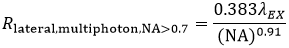
Equation 5 Lateral Resolution, Multiphoton LSM
and the axial resolution (Raxial,multiphoton) is:

Equation 6 Axial Resolution, Multiphoton LSM
These equations assume an objective NA > 0.7, which is true of virtually all multiphoton objectives.
The longer wavelength used for multiphoton excitation would lead one to believe (from Equation 5) that the resolution in multiphoton LSM, compared to confocal LSM, would be reduced roughly by a factor of two. For an ideal point object (i.e. a sub-resolution size fluorescent bead) the I2 signal dependence reduces the effective focal volume, more than offsetting the 2X increase in the focused illumination spot size.
We should note that the lateral and axial resolutions display a dependence on intensity. As laser power is increased, there is a corresponding increase in the probability of signal being generated within the diffraction-limited focal volume. In practice, the lateral resolution in a multiphoton microscope is limited by how tightly the illumination beam can be focused and is well approximated by Equation 5 at moderate intensities. Axial resolution will continue to degrade as excitation power is increased.
Image Display
Although we are not directly rendering an image, it is still important to consider the size of the image field, the number of pixels in which we are displaying our image (capture resolution) on the screen, and the lateral resolution of the imaging system. We use the lateral resolution because we are rendering an en face image. In order to faithfully display the finest features the optical system is capable of resolving, we must appropriately match resolution (capture and lateral) with the scan field. Our capture resolution must, therefore, appropriately sample the optical resolution.
In LSM, we typically rely on Nyquist sampling rules, which state that the pixel size should be the lateral resolution divided by 2.3. This means that if we take our 60X objective from earlier, the lateral resolution is 249 nm (Equation 2) and the pixel size in the displayed image should be 108 nm. Therefore, for a 1024 x 1024 pixel capture resolution, the scan field on the specimen would be ~111 μm x 111 μm. It should be noted that the 40X objective from our previous example would yield the exact same scan field (both objectives have the same NA) in the sample. The only difference between the two images is the angle at which we tilt our scanners to acquire the image.
It may not always be necessary to render images with such high resolution. We can always make the trade-off of image resolution, scan field, and capture resolution to create a balance of signal, sample longevity, and resolution in our images.
Considerations in Live Cell Imaging
One of LSM's greatest attributes is its ability to image living cells and tissues. Unfortunately, some of the by-products of fluorescence can be cytotoxic. As such, there is a delicate balancing act between generating high-quality images and keeping cells alive.
One important consideration is fluorophore saturation. Saturation occurs when increasing the laser power does not provide the expected concurrent increase in the fluorescence signal. This can occur when as few as 10% of the fluorophores are in the excited state.
The reason behind saturation is the amount of time a fluorophore requires to relax back down to the ground state once excited. While the fluorescence pathways are relatively fast (hundreds of ps to a few ns), this represents only one relaxation mechanism. Triplet state conversion and nonradiative decay require significantly longer relaxation times. Furthermore, re-exciting a fluorophore before it has relaxed back down to the ground state can lead to irreversible bleaching of the fluorophore. Cells have their own intrinsic mechanisms for dealing with the cytotoxicity associated with fluorescence, so long as excitation occurs slowly.
One method to reduce photobleaching and the associated cytotoxicity is through fast scanning. While reducing the amount of time the laser spends on a single point in the image will proportionally decrease the amount of detected signal, it also reduces some of the bleaching mechanisms by allowing the fluorophore to completely relax back to the ground state before the laser is scanned back to that point. If the utmost in speed is not a critical issue, one can average several lines or complete frames and build up the signal lost from the shorter integration time.
The longer excitation wavelength and non-descanned detection ability of multiphoton LSM give the ability to image deeper within biological tissues. Longer wavelengths are less susceptible to scattering by the sample because of the inverse fourth power dependence (I-4) of scattering on wavelength. Typical penetration depths for multiphoton LSM are 250 - 500 μm, although imaging as deep as 1 mm has been reported in the literature, compared to ~100 μm for confocal LSM.
Thorlabs recognizes that each imaging application has unique requirements.
If you have any feedback, questions, or need a quotation, please contact ImagingSales@thorlabs.com or call (703) 651-1700.
| Posted Comments: | |
Sylvie Le Guyader
(posted 2024-02-26 08:46:57.293) Hello
In this information webpage (https://www.thorlabs.com/newgrouppage9.cfm?objectgroup_id=10765), you state the equations for the resolution (axial and lateral) of a multiphoton system. Would you have a reference for these equations? What are the equations if the objective NA is higher than 0.7?
Thanks
Sylvie Le Guyader cdolbashian
(posted 2024-05-01 04:46:45.0) Thank you for reaching out to us with this inquiry. The information is gathered from the following paper: https://www.nature.com/articles/nbt899. I have contacted you directly to discuss from exactly where within this paper the information was interpreted. Additionally, the equations on the page are the ones which would be used with NA > 0.7. |